


添加时间:2024-07-11 18:05:23
我们知道g20可以很方便的指定优化算法是LM,GN还是Dog-Leg,比如g2o::OptimizationAlgorithmLevenberg* solver=new g2o::OptimizationAlgorithmLevenberg( solver_ptr )。但是Ceres如何指定呢?是在ceres::Solver::Options options;这个地方操作吗?
Solver::Options options;
options.trust_region_strategy_type=ceres::DOGLEG;
Ceres 非线性优化库广泛应用于SFM、SLAM和IMU定标等领域,是做计算机视觉绕不开的非线性优化开源库。官方文档当然是最全面的学习材料,但是也不容易短时间抓住重点,因此参考多个文章进行简单的总结。Ceres非线性优化需要四步:
要掌握Ceres 的使用,需要了解加黑部分的类和函数的意义。例如,一段IMU标定的优化代码,
    ......
    ceres::Problem problem;
    for (int i = 0, t_idx = 0; i < n_static_pos - 1; i++) {

        Eigen::Matrix<T, 3, 1> g_vs_pos0 = static_acc_means[i].data(),
                               g_vs_pos1 = static_acc_means[i + 1].data();

        g_versor_pos0 /= g_vs_pos0.norm();
        g_versor_pos1 /= g_vs_pos1.norm();

        int gyro_idx0 = -1,
            gyro_idx1 = -1;

        // Assume monotone signal time
        ......

        DataInterval gyro_interval(gyro_idx0, gyro_idx1);

        //  Add acc calibration cost function
        //  Create 函数的定义见后面
        ceres::CostFunction *cost_func
                     = MultiPos_GyroResidual<T>::Create(g_versor_pos0,
                                                       g_versor_pos1,
                                                       calib_gyro_samples_,
                                                       gyro_interval,
                                                       gyro_dt_);
        problem.AddResidualBlock(cost_func,
                                 nullptr /* squared loss */,
                                 gyro_calib_params.data());

    }

    ceres::Solver::Options options;
    options.linear_solver_type = ceres::DENSE_QR;
    options.max_num_iterations = max_num_iterations_;

    ceres::Solve(options, &problem, &summary);  // 优化问题求解

    // 优化结果
    gyro_calib_ = CalibratedTriad_<T>(
            gyro_calib_params[0], gyro_calib_params[1], gyro_calib_params[2],
            gyro_calib_params[3], gyro_calib_params[4], gyro_calib_params[5],
            gyro_calib_params[6], gyro_calib_params[7], gyro_calib_params[8],
            T(gyro_bias(0)), T(gyro_bias(1)), T(gyro_bias(2)),
            T(gyro_G(0)), T(gyro_G(1)), T(gyro_G(2)),
            T(gyro_G(3)), T(gyro_G(4)), T(gyro_G(5)),
            T(gyro_G(6)), T(gyro_G(7)), T(gyro_G(8))
    );
    ......
下面介绍使用ceres需要掌握的几个类和函数
Ceres的求解过程包括构建立最小二乘和求解最小二乘问题两部分,其中构建最小二乘问题的相关方法均包含在Ceres::Problem类中,涉及的成员函数主要包括:
2.1 Problem::AddResidualBlock()
用于向 Problem 类传递残差模块的信息,函数原型如下,传递的参数主要包括:代价函数模块、损失函数模块 和 参数模块;
ResidualBlockId Problem::AddResidualBlock(
   CostFunction *cost_function,
   LossFunction *loss_function,
   const vector<double *> parameter_blocks
)

ResidualBlockId Problem::AddResidualBlock(
   CostFunction *cost_function,
   LossFunction *loss_function,
   double *x0, double *x1, ...
)
(1) 代价函数模块:
包含了参数模块的维度信息,内部使用仿函数定义误差函数的计算方式。AddResidualBlock() 函数会检测传入的参数模块是否和代价函数模块中定义的维数一致,维度不一致时程序会强制退出。
(2) 损失函数模块:
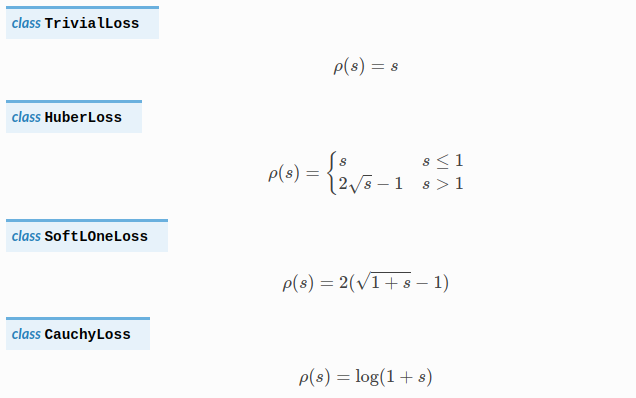
用于处理参数中含有野值的情况,避免错误量测对估计的影响,常用参数包括 HuberLoss、CauchyLoss 等,更多参见API;该参数可以取 NULL 或 nullptr,此时损失函数为单位函数。
(3) 参数模块:
待优化的参数,可一次性传入所有参数的指针容器 vector<double*> 或 依次传入所有参数的指针double*。
用户在调用 AddResidualBlock() 时其实已经隐式地向 Problem 传递了参数模块,但在一些情况下,需要用户显式地向 Problem 传入参数模块(通常出现在需要对优化参数进行重新参数化的情况,因为这个时候,优化的参数已经变了)。
Probelm 还提供了其他关于 ResidualBlock 和 ParameterBlock 的函数,例如获取模块维数、判断是否存在模块、存在的模块数目等,完整参见ceres API:
// 设定对应的参数模块在优化过程中保持不变
void Problem::SetParameterBlockConstant(double *values)

// 设定对应的参数模块在优化过程中可变
void Problem::SetParameterBlockVariable(double *values)

// 设定优化上界下界
void Problem::SetParameterUpperBound(
  double *values, int index, double upper_bound
)
void Problem::SetParameterLowerBound(
  double *values, int index, double lower_bound
)

// 该紧跟在参数赋值后,在给定的参数位置求解Problem,
// 给出当前位置处的cost、梯度以及Jacobian矩阵;
bool Problem::Evaluate(
   const Problem::EvaluateOptions &options,
   double *cost, vector<double>* residuals,
   vector<double> *gradient, CRSMatrix *jacobian
)
与其他非线性优化工具包一样,ceres的性能很大程度上依赖于导数计算的精度和效率,微分求导效率决定梯度下降的的效率,也就是成本函数最小化的求解效率,在ceres中由为 CostFunction类负责,ceres提供了许多种 CostFunction模板,较为常用的包括以下三种:
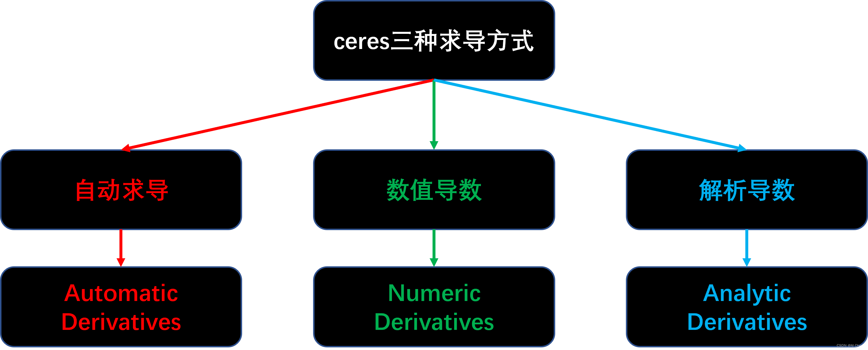
3.1 三种求导方式
(1) 自动导数(AutoDiffCostFunction)
由ceres自行决定导数的计算方式,最常用的求导方式,内部实现可参考该文章,具体使用参考文章。例如,AutoDiffCostFunction的使用,
static ceres::CostFunction *Create(
   const Eigen::Matrix<T1, 3, 1> &g_versor_pos0,
   const Eigen::Matrix<T1, 3, 1> &g_versor_pos1,
   const std::vector<TriadData_<T1> > &gyro_samples,
   const DataInterval &gyro_interval_pos01,
   T1 dt) {

      return (
         new ceres::AutoDiffCostFunction<MultiPos_GyroResidual, 3, 9>(
             new MultiPos_GyroResidual(g_versor_pos0,
                                       g_versor_pos1,
                                       gyro_samples,
                                       gyro_interval_pos01, dt)
         )
      );
}
(2) 数值导数(NumericDiffCostFunction)
当无法分析或使用自动微分计算导数时,应使用数值微分,如用一个外部库或函数时;但精度和计算效率不如自动导数和解析导数,因此不到不得已,官方并不建议使用该方法。
当使用数值微分时,至少使用中值差分;如果执行时间不是问题,或者目标函数难以确定良好的静态相对步长,建议使用Ridders方法,就是梯度法。
(3) 解析导数(SizedCostFunction)
当导数存在闭合解析形式时使用,用于可基于SizedCostFunction基类自行编写,但由于需要自行管理残差和雅克比矩阵,除非闭合解具有具有明显的精度和效率优势,否则同样不建议使用。
AutoDiffCostFunctio较为常用,下面进行详细说明。
3.2 AutoDiffCostFunction
官方推荐用户使用AutoDiffCostFunction,这是一个模板类,构造函数如下:
ceres::AutoDiffCostFunction< CostFunctor,           // 仿函数(functor)类型
                             int residualDim,       // 残差维数
                             int paramDim           // 参数维数(可以有多个)
                           > (CostFunctor* functor);// CostFunctor: 仿函数指针
CostFunctor仿函数
仿函数为struct或class,由于重载了()运算符,使得其能够具有和函数一样的调用行为,因此被称为仿函数。由于要实现仿函数功能,所以必须重载operator()运算符。
template<typename T1> struct MultiPos_GyroResidual {

    MultiPos_GyroResidual(const Eigen::Matrix<T1, 3, 1> &g_versor_pos0,
                          const Eigen::Matrix<T1, 3, 1> &g_versor_pos1,
                          const std::vector<TriadData_<T1> > &gyro_samples,
                          const DataInterval &gyro_interval_pos01,
                          T1 dt) :
            g_versor_pos0_(g_versor_pos0),
            g_versor_pos1_(g_versor_pos1),
            gyro_samples_(gyro_samples),
            interval_pos01_(gyro_interval_pos01),
            dt_(dt) {

    }
    // 重载括号,以求残差
    template<typename T2>
    bool operator()(const T2 *const params, T2 *residuals) const {

        CalibratedTriad_<T2> calib_triad;
        calib_triad = CalibratedTriad_<T2>(params[0], params[1], params[2],
                                           params[3], params[4], params[5],
                                           params[6], params[7], params[8],
                                           T2(0), T2(0), T2(0));
        std::vector<TriadData_<T2> > calib_gyro_samples;
        calib_gyro_samples.reserve(
          interval_pos01_.end_idx - interval_pos01_.start_idx + 1
        );

        for (int i = interval_pos01_.start_idx;
                 i <= interval_pos01_.end_idx; i++) {
            calib_gyro_samples.push_back(
              TriadData_<T2>(calib_triad.unbiasNormalize(gyro_samples_[i]))
            );
        }

        Eigen::Matrix<T2, 3, 3> rot_mat;
        integrateGyroInterval(calib_gyro_samples, rot_mat, T2(dt_));
        // 求相邻位置的陀螺仪读数残差
        Eigen::Matrix<T2, 3, 1> diff =
            rot_mat.transpose() * g_versor_pos0_.template cast<T2>() -
            g_versor_pos1_.template cast<T2>();

        residuals[0] = diff(0);
        residuals[1] = diff(1);
        residuals[2] = diff(2);

        return true;
    }

    static ceres::CostFunction *Create(
            const Eigen::Matrix<T1, 3, 1> &g_versor_pos0,
            const Eigen::Matrix<T1, 3, 1> &g_versor_pos1,
            const std::vector<TriadData_<T1> > &gyro_samples,
            const DataInterval &gyro_interval_pos01,
            T1 dt) {

       return (
         // AutoDiffCostFunction 自动求导
         new ceres::AutoDiffCostFunction<MultiPos_GyroResidual, 3, 9>(
             // MultiPos_GyroResidual重载了()以求残差
             new MultiPos_GyroResidual(g_versor_pos0,
                                       g_versor_pos1,
                                       gyro_samples,
                                       gyro_interval_pos01, dt)
         )
      );
    }

    const Eigen::Matrix<T1, 3, 1> g_versor_pos0_, g_versor_pos1_;
    const std::vector<TriadData_<T1> > gyro_samples_;
    const DataInterval interval_pos01_;
    const T1 dt_;
};
求解最小二乘问题,需要首先构建一个ceres::Problem对象,利用AddResidualBlock向其中添加残差模块。然后通过ceres::Solve函数是求解。函数原型如下:
void Solve(
   const Solver::Options& options, // 求解的核心,控制消元顺序、分解方法、收敛精度
   Problem* problem,               // 构建的最小二乘问题
   Solver::Summary* summary        // 存储求解过程中的相关信息,不影响求解器性能
)
problem参数已经介绍过,summary参数存储求解过程中的相关信息,相对简单,Solver::Options含有的参数种类繁多,是使用过程中需要着重设置的部分。这里列出一些常用参数:
minimizer_type:迭代求解方法,可选LINEAR_SEARCH或TRUST_REGION(默认)。由于大多数情况选择LM或DOGLEG方法,因此该选项默认;trust_region_strategy_type:信赖域策略,可选LEVENBERG_MARQUARDT(默认)或DOGLEG,没有高斯牛顿选项;linear_solver_type:信赖域方法中,求解线性方程组所使用的求解器类型,默认为DENSE_QR;linear_solver_ordering:线性方程求解器的消元顺序,默认为NULL(即由Ceres自行决定);在以BA为代表对消元顺序有特殊要求的应用中,可以通过成员函数reset设定消元顺序;min_linear_solver_iteration/max_linear_solver_iteration:意义如名,默认为0/500,一般不需要更改;max_num_iterations:求解器的最大迭代次数;max_solver_time_in_seconds:求解器的最大运行秒数;num_threads:Ceres求解时使用的线程数;minimizer_progress_to_stdout:是否向终端输出优化过程信息;在实际应用中,对最终求解性能影响最大的就是linear_solver_type和线程数num_threads,如果发现最后的求解精度或求解效率不能满足要求,应首先尝试更换这两个参数。ceres solver定义了7种线性求解器:
注意:系数矩阵如果不满足分解方法对应前提条件(可逆、对称、正定等)时,可能会求解失败。
Ceres消元顺序的设置由linear_solver_ordering的reset函数完成,该函数接受参数为ParameterBlockOrdering对象。该对象将所有待优化参数存储为带标记(ID)的组(Group),ID小的Group在求解线性方程的过程中会被首先消去。因此,需要做的第一个工作是调用其成员函数AddElementToGroup将参数添加到对应ID的Group中,函数原型为:
bool ParameterBlockOrdering::AddElementToGroup(
    const double *element,  // 变量数组的指针
    const int group         // 组ID为非负整数,如果该Id对应的Group不存在,则自动创建
)
例如,
ceres::ParameterBlockOrdering* order = new ceres::ParameterBlockOrdering();

// set all points in ordering to 0
for(int i = 0; i < num_points; i++){
    order->AddElementToGroup(points + i * point_block_size, 0);
}
// set all cameras in ordering to 1
for(int i = 0; i < num_cameras; i++){
    order->AddElementToGroup(cameras + i * camera_block_size, 1);
}
该例子中,所有路标点被分到了ID=0组,而所有相机位姿被分到了ID=1组,因此在线性方程组的求解中,所有路标点会变首先SCHUR消元。接下来,就可以使用reset函数制定线性求解器的消元顺序了:
// set ordering in options
options->linear_solver_ordering.reset(ordering);
该选型默认为false,即根据vlog设置等级的不同,只会在向STDERR中输出错误信息;若设置为true则会向程序的运行终端输出优化过程的所有信息,根据所设置优化方法的不同,输出的参数亦不同。求解器设置例子:
ceres::Solver::Options options;
options.linear_solver_type = ceres::DENSE_SCHUR; // 使用DENSE_SCHUR分解
options.minimizer_progress_to_stdout = true;     // 输出优化过程信息
ceres是经常会用到的非线性优化库,之前看官网的文档总是不能深入,最近看了一个IMU 的定标项目,里面就用到了这个优化库。感觉看网络上的解析文章并结合具体项目更容易理解,一开始就看官方文档容易陷入很多不着急的细节中。先看简单文章和项目,熟悉上手掌握大概后,有需要再去看文档,有的放矢,效率更高。
参考:
单个无人机三维路径规划问题及其建模_IT猿手的博客-CSDN博客
参考文献:
[1]胡观凯,钟建华,李永正,黎万洪.基于IPSO-GA算法的无人机三维路径规划[J].现代电子技术,2023,46(07):115-120
高尔夫优化算法(Golf Optimization Algorithm,GOA)由Montazeri Z等人于2023年提出,该算法模拟高尔夫运动过程中的球员击打高尔夫所采取的战术策略,能够有效平衡全局搜索和局部搜索的能力。
https://blog.csdn.net/weixin_46204734/article/details/132939196
参考文献:
[1]Montazeri Z, Niknam T, Aghaei J, Malik OP, Dehghani M, Dhiman G. Golf Optimization Algorithm: A New Game-Based Metaheuristic Algorithm and Its Application to Energy Commitment Problem Considering Resilience. Biomimetics. 2023; 8(5):386. Biomimetics | Free Full-Text | Golf Optimization Algorithm: A New Game-Based Metaheuristic Algorithm and Its Application to Energy Commitment Problem Considering Resilience
(1)部分代码
close all
clear
clc
addpath('https://www.zhihu.com/question/Algorithm/')%添加算法路径
warning off;
%% 三维路径规划模型定义
global startPos goalPos N
N=2;%待优化点的个数(可以修改)
startPos=[10, 10, 80]; %起点(可以修改)
goalPos=[80, 90, 150]; %终点(可以修改)
SearchAgents_no=30; % 种群大小(可以修改)
Function_name='F1'; %F1:随机产生地图 F2:导入固定地图
Max_iteration=50; %最大迭代次数(可以修改)
% Load details of the selected benchmark function
[lb,ub,dim,fobj]=Get_Functions_details(Function_name);
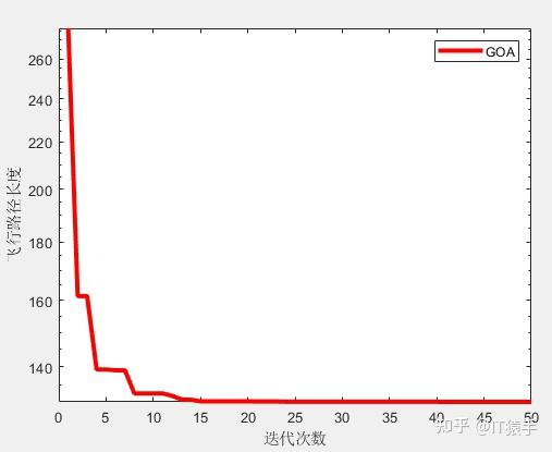
[Best_score,Best_pos,curve]=GOA(SearchAgents_no,Max_iteration,lb,ub,dim,fobj);%算法优化求解
AlgorithmName='GOA';%算法名字
figure
semilogy(curve,'Color','r','linewidth',3)
xlabel('迭代次数');
ylabel('飞行路径长度');
legend(AlgorithmName)
display(['算法得到的最优适应度: ', num2str(Best_score)]);
Position=[Best_pos(1:dim/3); Best_pos(1+dim/3:2*(dim/3)); Best_pos(1+(2*dim/3):end)]'; %优化点的XYZ坐标(每一行是一个点)
plotFigure(Best_pos,AlgorithmName)%画最优路径
(2)部分结果
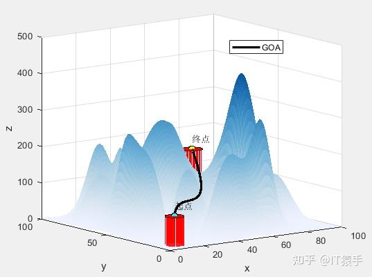
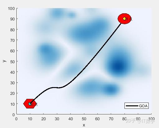
无人机飞行路径坐标:
   1.0000000e+01   1.0000000e+01   8.0000000e+01
   1.1195509e+01   1.1522382e+01   8.1134937e+01
   1.2336219e+01   1.2941987e+01   8.2210564e+01
   1.3423955e+01   1.4262310e+01   8.3228946e+01
   1.4460544e+01   1.5486846e+01   8.4192142e+01
   1.5447811e+01   1.6619089e+01   8.5102217e+01
   1.6387583e+01   1.7662536e+01   8.5961231e+01
   1.7281684e+01   1.8620681e+01   8.6771246e+01
   1.8131942e+01   1.9497019e+01   8.7534326e+01
   1.8940182e+01   2.0295045e+01   8.8252532e+01
   1.9708230e+01   2.1018255e+01   8.8927926e+01
   2.0437912e+01   2.1670143e+01   8.9562570e+01
   2.1131053e+01   2.2254205e+01   9.0158527e+01
   2.1789480e+01   2.2773936e+01   9.0717858e+01
   2.2415019e+01   2.3232830e+01   9.1242626e+01
   2.3009496e+01   2.3634383e+01   9.1734893e+01
   2.3574735e+01   2.3982091e+01   9.2196721e+01
   2.4112565e+01   2.4279447e+01   9.2630172e+01
   2.4624809e+01   2.4529948e+01   9.3037307e+01
   2.5113295e+01   2.4737088e+01   9.3420191e+01
   2.5579848e+01   2.4904362e+01   9.3780883e+01
   2.6026294e+01   2.5035266e+01   9.4121447e+01
   2.6454458e+01   2.5133295e+01   9.4443945e+01
   2.6866168e+01   2.5201943e+01   9.4750438e+01
   2.7263249e+01   2.5244706e+01   9.5042989e+01
   2.7647526e+01   2.5265079e+01   9.5323660e+01
   2.8020826e+01   2.5266557e+01   9.5594514e+01
   2.8384974e+01   2.5252635e+01   9.5857611e+01
   2.8741797e+01   2.5226808e+01   9.6115015e+01
   2.9093120e+01   2.5192572e+01   9.6368787e+01
   2.9440769e+01   2.5153420e+01   9.6620990e+01
   2.9786571e+01   2.5112850e+01   9.6873686e+01
   3.0132351e+01   2.5074355e+01   9.7128936e+01
   3.0479935e+01   2.5041430e+01   9.7388803e+01
   3.0831149e+01   2.5017571e+01   9.7655350e+01
   3.1187818e+01   2.5006274e+01   9.7930637e+01
   3.1551770e+01   2.5011032e+01   9.8216728e+01
   3.1924829e+01   2.5035341e+01   9.8515684e+01
   3.2308821e+01   2.5082696e+01   9.8829568e+01
   3.2705574e+01   2.5156593e+01   9.9160441e+01
   3.3116912e+01   2.5260526e+01   9.9510366e+01
   3.3544661e+01   2.5397990e+01   9.9881405e+01
   3.3990647e+01   2.5572481e+01   1.0027562e+02
   3.4456697e+01   2.5787494e+01   1.0069507e+02
   3.4944635e+01   2.6046523e+01   1.0114183e+02
   3.5456289e+01   2.6353064e+01   1.0161794e+02
   3.5993484e+01   2.6710612e+01   1.0212548e+02
   3.6558045e+01   2.7122662e+01   1.0266651e+02
   3.7151799e+01   2.7592710e+01   1.0324308e+02
   3.7776572e+01   2.8124249e+01   1.0385727e+02
   3.8434190e+01   2.8720776e+01   1.0451113e+02
   3.9126478e+01   2.9385785e+01   1.0520672e+02
   3.9855263e+01   3.0122772e+01   1.0594611e+02
   4.0622370e+01   3.0935231e+01   1.0673137e+02
   4.1429625e+01   3.1826658e+01   1.0756454e+02
   4.2278854e+01   3.2800548e+01   1.0844769e+02
   4.3171884e+01   3.3860396e+01   1.0938289e+02
   4.4110539e+01   3.5009697e+01   1.1037220e+02
   4.5096647e+01   3.6251945e+01   1.1141768e+02
   4.6132032e+01   3.7590637e+01   1.1252139e+02
   4.7218521e+01   3.9029268e+01   1.1368540e+02
   4.8357940e+01   4.0571332e+01   1.1491176e+02
   4.9552115e+01   4.2220324e+01   1.1620254e+02
   5.0802871e+01   4.3979740e+01   1.1755980e+02
   5.2112034e+01   4.5853074e+01   1.1898560e+02
   5.3481431e+01   4.7843822e+01   1.2048201e+02
   5.4912887e+01   4.9955480e+01   1.2205109e+02
   5.6408228e+01   5.2191541e+01   1.2369489e+02
   5.7969280e+01   5.4555501e+01   1.2541548e+02
   5.9597869e+01   5.7050855e+01   1.2721493e+02
   6.1295822e+01   5.9681099e+01   1.2909529e+02
   6.3064963e+01   6.2449727e+01   1.3105863e+02
   6.4907119e+01   6.5360235e+01   1.3310701e+02
   6.6824115e+01   6.8416117e+01   1.3524250e+02
   6.8817778e+01   7.1620868e+01   1.3746714e+02
   7.0889934e+01   7.4977985e+01   1.3978301e+02
   7.3042408e+01   7.8490961e+01   1.4219217e+02
   7.5277026e+01   8.2163292e+01   1.4469668e+02
   7.7595615e+01   8.5998474e+01   1.4729860e+02
   8.0000000e+01   9.0000000e+01   1.5000000e+02
(一)基于高尔夫优化算法GOA求解无人机三维路径规划研究(MATLAB) - 哔哩哔哩 (bilibili.com)
在使用Ceres库进行非线性优化(二)中介绍了三种求导方式。本文就最小化罗森布罗克函数再次进行示例。并给出与之前略有差别的实现方式。
与一般通用的非线性优化不同,此类问题主要是求一阶导数后,就可以计算出相关最值点,因此使用下述函数来创建问题。
ceres::GradientProblem problem(Rosenbrock::Create());
//Rosenbrock为自定义的结构体
#include "ceres/ceres.h"

// f(x,y)=(1-x)^2 + 100(y - x^2)^2;
struct Rosenbrock {
  template <typename T>
  bool operator()(const T* parameters, T* cost) const {
    const T x = parameters[0];
    const T y = parameters[1];
    cost[0] = (1.0 - x) * (1.0 - x) + 100.0 * (y - x * x) * (y - x * x);
    return true;
  }
  static ceres::FirstOrderFunction* Create() {
    constexpr int kNumParameters = 2;
    return new ceres::AutoDiffFirstOrderFunction<Rosenbrock,
                                                 kNumParameters>(new Rosenbrock);
  }
};
int main(int argc, char** argv) {

  double parameters[2] = {-1.2, 1.0};
  ceres::GradientProblemSolver::Options options;
  options.minimizer_progress_to_stdout = true;

  ceres::GradientProblemSolver::Summary summary;

  ceres::GradientProblem problem(Rosenbrock::Create());

  ceres::Solve(options, problem, parameters, &summary);
  std::cout << summary.FullReport() << "\
";
  std::cout << "Initial x: " << -1.2 << " y: " << 1.0 << "\
";
  std::cout << "Final   x: " << parameters[0] << " y: " << parameters[1]
            << "\
";
  return 0;
}
如果函数内部调用了别的库的函数,不知道具体的实现细节,可以使用numeric differentiation来求导。
此时函数定义如下:
// f(x,y)=(1-x)^2 + 100(y - x^2)^2;
struct Rosenbrock {
  bool operator()(const double* parameters, double* cost) const {
    const double x = parameters[0];
    const double y = parameters[1];
    cost[0] = (1.0 - x) * (1.0 - x) + 100.0 * (y - x * x) * (y - x * x);
    return true;
  }

  static ceres::FirstOrderFunction* Create() {
    constexpr int kNumParameters = 2;//参数的数量
    return new ceres::NumericDiffFirstOrderFunction<Rosenbrock,
                                                    ceres::CENTRAL,//使用中心差分(Central Difference)的数值微分方法
                                                    kNumParameters>(
        new Rosenbrock);
  }
};
#include "ceres/ceres.h"
// f(x,y)=(1-x)^2 + 100(y - x^2)^2;
struct Rosenbrock {
  bool operator()(const double* parameters, double* cost) const {
    const double x = parameters[0];
    const double y = parameters[1];
    cost[0] = (1.0 - x) * (1.0 - x) + 100.0 * (y - x * x) * (y - x * x);
    return true;
  }
  static ceres::FirstOrderFunction* Create() {
    constexpr int kNumParameters = 2;
    return new ceres::NumericDiffFirstOrderFunction<Rosenbrock,
                                                    ceres::CENTRAL,
                                                    kNumParameters>(
        new Rosenbrock);
  }
};
int main(int argc, char** argv) {

  double parameters[2] = {-1.2, 1.0};
  ceres::GradientProblemSolver::Options options;
  options.minimizer_progress_to_stdout = true;
  ceres::GradientProblemSolver::Summary summary;

  ceres::GradientProblem problem(Rosenbrock::Create());

  ceres::Solve(options, problem, parameters, &summary);

  std::cout << summary.FullReport() << "\
";
  std::cout << "Initial x: " << -1.2 << " y: " << 1.0 << "\
";
  std::cout << "Final   x: " << parameters[0] << " y: " << parameters[1]
            << "\
";
  return 0;
}
自动求导带来了简便,但是如果参数数量太多,会带来很大的计算开销,如在使用自动求导时,使用ceres::CENTRAL,尽管中心差分相对于其他数值微分方法的优点是它提供了相对较高的数值稳定性和精度。它使用两个取样点,从而减小了舍入误差的影响。然而,它的计算成本可能相对较高,因为它需要两次函数评估。
所以如果能够通过定义ceres::FirstOrderFunction,可以更好的进行非线性优化。
此时函数定义如下:
// f(x,y)=(1-x)^2 + 100(y - x^2)^2;
class Rosenbrock final  : public ceres::FirstOrderFunction {
  public:
    ~Rosenbrock() override {}

    bool Evaluate(const double* parameters,
                           double* cost,
                           double* gradient) const override {
       const double x = parameters[0];
       const double y = parameters[1];

       cost[0] = (1.0 - x) * (1.0 - x) + 100.0 * (y - x * x) * (y - x * x);
       if (gradient) {
         gradient[0] = -2.0 * (1.0 - x) - 200.0 * (y - x * x) * 2.0 * x;
         gradient[1] = 200.0 * (y - x * x);
       }
      return true;
   }

   int NumParameters() const override { return 2; }
};

/*
class Rosenbrock final  : public ceres::FirstOrderFunction
final 关键字防止其他类继承 Rosenbrock 类。如果某个类不再被设计为基类,而且你不希望它有任何派生类,可以将其标记为 final,以确保该类的继承链终止。

override 关键字用于显式声明派生类中的成员函数将覆盖(重写)基类中的虚函数。在你提供的代码中,override 关键字用于表示 ~Rosenbrock() 函数是对基类中虚析构函数 virtual ~Rosenbrock() 的重写。

int NumParameters() const override{ return 2; }
代码表示派生类中的 NumParameters 函数重写了基类中的同名虚函数,并在被调用时返回固定的整数值 2。在 Ceres Solver 中,这个函数通常用于指定优化问题的参数数量。

*/
#include "ceres/ceres.h"

// f(x,y)=(1-x)^2 + 100(y - x^2)^2;
class Rosenbrock final : public ceres::FirstOrderFunction {
 public:
  bool Evaluate(const double* parameters,
                double* cost,
                double* gradient) const override {
    const double x = parameters[0];
    const double y = parameters[1];
    cost[0] = (1.0 - x) * (1.0 - x) + 100.0 * (y - x * x) * (y - x * x);
    if (gradient) {
      gradient[0] = -2.0 * (1.0 - x) - 200.0 * (y - x * x) * 2.0 * x;
      gradient[1] = 200.0 * (y - x * x);
    }
    return true;
  }
  int NumParameters() const override { return 2; }
};
int main(int argc, char** argv) {

  double parameters[2] = {-1.2, 1.0};
  ceres::GradientProblemSolver::Options options;
  options.minimizer_progress_to_stdout = true;
  ceres::GradientProblemSolver::Summary summary;

  ceres::GradientProblem problem(new Rosenbrock());

  ceres::Solve(options, problem, parameters, &summary);
  std::cout << summary.FullReport() << "\
";
  std::cout << "Initial x: " << -1.2 << " y: " << 1.0 << "\
";
  std::cout << "Final   x: " << parameters[0] << " y: " << parameters[1]
            << "\
";
  return 0;
}
在上述示例中Automatic Differentiation和Numeric Differentiation都是使用结构体形式,在定义时:
//Automatic Differentiation
static ceres::FirstOrderFunction* Create() {
    constexpr int kNumParameters = 2;
    return new ceres::AutoDiffFirstOrderFunction<Rosenbrock,
                                                 kNumParameters>(new Rosenbrock);
  }

// Numeric Differentiation
 static ceres::FirstOrderFunction* Create() {
    constexpr int kNumParameters = 2;
    return new ceres::NumericDiffFirstOrderFunction<Rosenbrock,
                                                    ceres::CENTRAL,
                                                    kNumParameters>(
        new Rosenbrock);
  }
而对于手动提供一阶导的Analytic Derivatives:
// Analytic Derivatives
if (gradient) {
         gradient[0] = -2.0 * (1.0 - x) - 200.0 * (y - x * x) * 2.0 * x;
         gradient[1] = 200.0 * (y - x * x);
       }
      return true;
   }

   int NumParameters() const override { return 2; }
在主函数构建问题时:
//Automatic Differentiation
 ceres::GradientProblem problem(Rosenbrock::Create());

// Numeric Differentiation
  ceres::GradientProblem problem(Rosenbrock::Create());

// Analytic Derivatives
  ceres::GradientProblem problem(new Rosenbrock());
由上述可知,使用Automatic Differentiation和Numeric Differentiation其对象的构建在creat()里面已经实现,所以在构建问题时,直接调用就行problem(Rosenbrock::Create())。而在Analytic Derivatives 则需要生成对象problem(new Rosenbrock())。
地址:海南省海口市电话:0898-08980898传真:0898-1230-5678
Copyright © 2012-2018 耀世娱乐-耀世注册登录入口 版权所有ICP备案编号:琼ICP备xxxxxxxx号